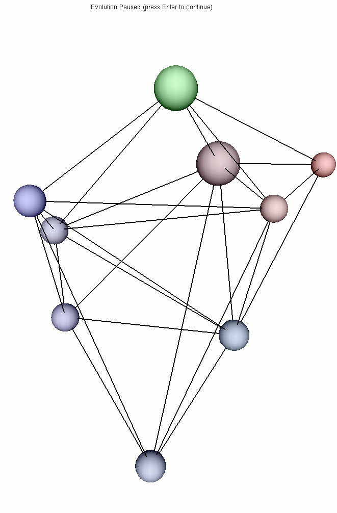
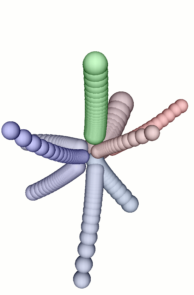
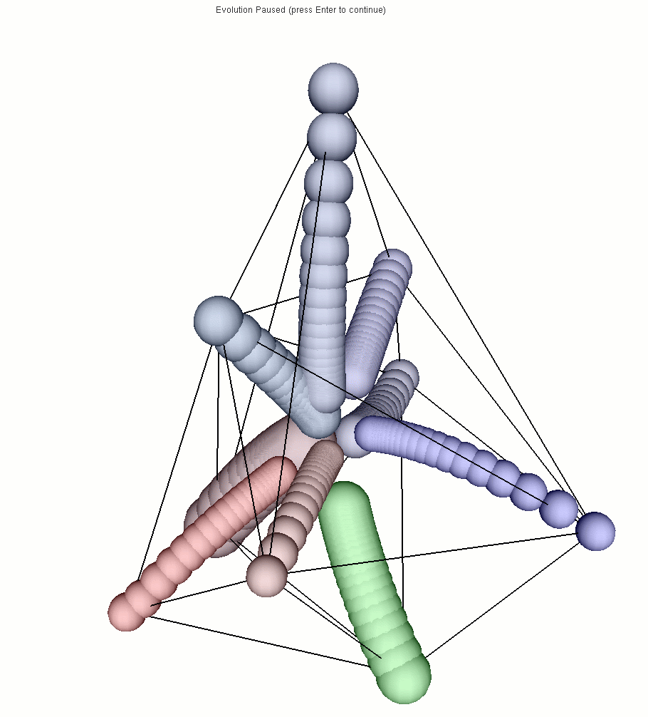
This simple model was developped jointly with Pierre Barbier de Reuille to validate the use of Delaunay collection types. This model does not correspond to any "natural" system. It is just a (formal) example of an interacting set of entities localized in a 3D space, such that the interactions both depend on the position of the entities and make these positions evolve.
Each sphere in the picture below corresponds to a cell attracted
by its neighboring cells by a kind of spring force. The neighborhood of a
cell is computed dynamically using a Delaunay graph built from the cells
position. At each time step, this neighborhood can change due
to the cell movements. In MGS, the Delaunay collection type is a type
constructor corresponding to the building of collection with a neighborhood
computed from the position of the elements in a d-dimensional space.
The first picture is the initial state and shows the neighborhood using
links between the cells. The second picture shows the final state, when
the system has reached an equilibrium (each "tube" in this picture represents
the successive positions of a cell). The last picture shows the final
state from another point of view (the links represent the neighborhood
in the initial state).


Click to enlarge the view.
|
specifying the cell system
|
|
| record Position
= {x, y, z };; record Cell = Position + {l};; delaunay(3) D3 = \e.if Position(e) then (e.x, e.y, e.z) else ?("bad element type for D3 delaunay type") fi ;; |
A cell is represented as a record
containing the fields x, y and z which represent
the position of the cell in 3D, and a field l which represents the
stiffness of the cell spring. To define a Delaunay collection type in MGS, one has to give a function that extract a position in an euclidean space from the element in the collection. Here the function that defines the Delaunay type D3 simply checks if the element has the good type and extract the position from the record fields to return a sequence of three elements (because the Delaunay is done in 3D). |
| epsilon := 0.05;; K := 1.0;; |
The parameter epsilon
is the fragment of the force that is converted into an elementary displacement.
For the sake of the simpliciy, we do not integrate the force exercised on
each cell to have a speed and then a displacement but we consider simply that
a part of the computed force is converted directly into a displacement. This
makes the model unrealistic from a physical point of view but does not changes
fundamentally the computations done. The parameter K is used to control globallythe spring stiffness. |
| fun interaction(ref, src) = if(Cell(ref) && Cell(src)) then ( let X = ref.x - src.x and Y = ref.y - src.y and Z = ref.z - src.z and L = ref.l + src.l in let dist = sqrt(X*X+Y*Y+Z*Z) in let force = 0.0-K*(dist-L)/dist in {x=X*force, y = Y*force, z = Z*force} ) else ?("Error : bad argument type for interaction/2"); ?(ref); ?(src); ?("Et voil� ...") fi ;; |
This function computes the interaction between
a cell ref and one of its neighbor src. It simply computes
the distance between the two cell and then the corresponding force exerced
by the spring. The record returned correspond to the force vector. |
| fun add(u, v, e) = u + { x = u.x + e*v.x, y = u.y + e*v.y, z = u.z + e*v.z } ;; fun sum(x, u, acc) = add(acc, interaction(x,u), epsilon) ;; fun id(x) = x ;; |
Function add correspond to the vector addition,
where the vector are represented as records. The function sum is used in the neighborsfold operator in the transformation below. neighborsfold is a fold operator that iterates over the neighbors of an element in a collection. See here for a description of neighborsfold. The operator + between record computes the asymetric merge of the fields of its two arguments (the priority is given to the right argument). |
| trans H = { x => add(x,neighborsfold(sum(x), id, {x=0,y=0,z=0, l=x.l}, x), epsilon) };; |
The transformation H simply iterates for
each element in the collection, the sum of the neighbors contribution. |
|
computing an initial state |
|
| pre_init := {x = 15.0, y = 6.0, z = 0.0, color = "Color<1.0, 0, 0>", l = 1.0}, {x = 3.0, y = 10.0, z = 8.0, color = "Color<0, 1.0, 0>", l = 1.5}, {x = -6.0, y = 2.0, z = 12.0, color = "Color<0, 0, 1.0>", l = 1.0}, {x = 7.0, y = 7.0, z = -6.0, color = "Color<0.5, 0.1, 0.2>", l = 2.0}, {x = 10.0, y = 2.0, z = 6.0, color = "Color<0.8, 0.3, 0.3>", l = 1.0}, {x = 8.0, y = -8.0, z = -2.0, color = "Color<0.1, 0.3, 0.7>", l = 1.3}, {x = 1.0, y = -19.0, z = -2.0, color = "Color<0.2, 0.3, 0.7>", l = 1.3}, {x = -8.0, y = 1.0, z = -7.0, color = "Color<0.3, 0.3, 0.7>", l = 1.3}, {x = -7.0, y = -7.0, z = -7.0, color = "Color<0.2, 0.2, 0.8>", l = 1.3} ;; init := delaunayfy(D3:(), map(bruit(1.0), pre_init)) ;; |
To build an initial state we
transform a sequence of records representing the cells into a delaunay using
the primitive delaunayfy. The field color contains a string used in the graphical description of the cell to specify its color. |
|
outputing the graphical description |
|
| outfile := "tmp.moving1.imo";; fun show_line(a, b, acc) = ( outfile << "Polyline { PointList [ <" + a.x + ", " << a.y << ", " << a.z << ">, <" << b.x << ", " << b.y << ", " << b.z << "> ]}\n"; acc ) ;; trans show_edge = { x => (neighborfold(show_line(x), id, 0, x); x) } ;; |
The following functions are
used to writte in a file a 3D graphical description of the picture above.
The 3D description language is described here. The graphical description of the system state is outputed in the file outfile. The function show_line output the description of a line joining the two cell given as an argument. The + operator between a string and any values computes simply the concatenation of this string with the text representation of this value. For instance, "toto" + (3*4) evaluates to the string "toto12". This function is used in the transformation show_edge that shows the edges between two neighboring cells. |
| fun showcell(a) = "Translated { Translation <" + a.x + ", " + a.y + ", " + a.z + "> Geometry Sphere { Radius " + a.l + " Slices 16 Stacks 16 " + a.color + "} }" ;; |
The function show_cell returns a string
specifying the graphical representation of a cell : a sphere at some position
in space. |
| cpt := -1;; fun show(f, c) = ( cpt := 1+cpt; if 0 == cpt % 11 then ( if (cpt == 0) then show_edge(c) else 0 fi; print_coll(f, c, showcell, "Group { GeometryList [\n\t", ",\n\t", "\n] }\n\nCommand Pause\n\n")) else 0 fi) ;; fun evol(c) = (show("tmp.moving1.imo", c); H(c)) ;; evol[300](init) ;; system("imoview tmp.moving1.imo") ;; |
A global counter is used to output
a description of the system only each 11 evolution steps. See here a description of the predefined MGS function print_coll. The function show return a non-used value. The edges are showed only for the initial state. An evolution step consist in outputing the graphical description of the cells and making one evolution step of the system. Evolution steps are iterated 300 times. At the end, the graphical viewer is launched as an external process with the output file as an argument. |
| Back
to top |
MGS examples index |
MGS home page |

Pictures, graphics and animations are licensed under a Creative Commons License.
|
|