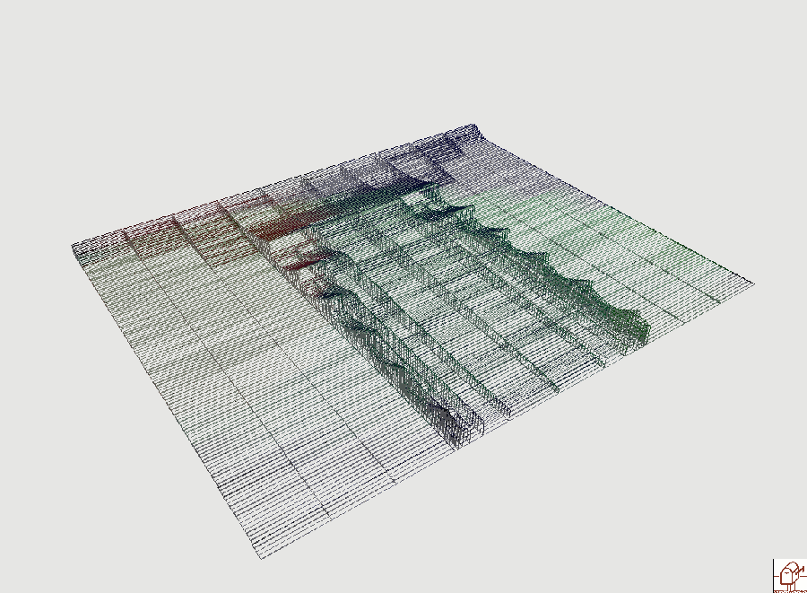
An MGS Gallery : Turing reaction-diffusion driving the cell division in a filament in MGS

This picture visualizes a Turing-like reaction-diffusion process on a line of cells, but one of the two chemicals is used as a trigger of the cell division. When its level is above a given threshold, the cell divides into two cells and the concentration in the two daughter cells is also divided. This process does not mimic an identified natural phenomena but is used as an example of some kind of physico-chemical process taking place in an expanding media.

In the visualization below, the complete evolution of the filement is show. An elementary bloc corresponds to one cell, the line of cells is in the screen plane and the time is directed toward you. The height of a block is proportional to the quantity of the triggering chemicals present in the corresponding cell. The width of the daughter cells are divided by two, so a lineage corresponds to a parallel strip directed toward you. The data produced by the MGS simulation are written in a file using the TEOM format. This language is used to describe 3D scenes that are later rendered using the ImoView front-end (which is part of the MGS distribution).

The corresponding MGS program

*specifying the Turing diffusion-reaction and the cell division*
`trans init = { x => { a = 3.5 + random(1.0) -0.5, b = 4.0, beta = 12.0 + random(0.1) - 0.05, size = 16 }; };; NbCell := 20;; filement0 := init(iota(NbCell, ():seq));;`	The filemant of cell is represented by a sequence of records; a record represents the state of one cell. Such a record has four fields: the fields `a` and `b` correspond to the concentration in morphogen a and b. The field `beta` is a constant used in the reaction-diffusion and that fluctuates a little randomly between the cells. The field `size` records the size of a cell. We start with 20 cells and the initial filament is made by applying the transformation `init` (which replaces each element `x` in a sequence by a record described as above) to a sequence made with the function `iota.` This function is reminiscent of the iota function in `APL` and builds a sequence of increasing integers.
`rsp := 1.0/16.0;; diff1 := 0.25;; diff2 := 0.0625;; fun da(a, b, la, ra) = rsp * (16.0 - ab) + diff1(la + ra - 2.0a);; fun db(a, b, beta, lb, rb) = rsp(ab - b - beta) + diff2(lb + rb - 2.0*b);;`	Some constant parameters of the reaction-diffusion process are defined. Function `da` and `db` computes the changes in morphogens a and b from the actual concentration of a cell and the concentrations of the left and right neighbors.
trans TuringSplit = { x / x.b > 8 => { a = x.a/2, b = x.b/2, beta = x.beta, size = x.size/2}, { a = x.a/2, b = x.b/2, beta = x.beta, size = x.size - x.size/2}; x / leftq(x) & rightq(x) => { a = x.a + da(x.a, x.b, left(x).a, right(x).a), b = max(0.0, x.b + db(x.a, x.b, x.beta, left(x).b, right(x).b)), beta = x.beta, size = x.size }; x / ~leftq(x) => { a = x.a + da(x.a, x.b, 0, right(x).a), b = max(0.0, x.b + db(x.a, x.b, x.beta, 0, right(x).b)), beta = x.beta, size = x.size }; x / ~rightq(x) => { a = x.a + da(x.a, x.b, left(x).a, 0), b = max(0.0, x.b + db(x.a, x.b, x.beta, left(x).b, 0)), beta = x.beta, size = x.size }; };;	The transformation `TuringSplit` computes the evolution of the filament. Each cell `x` is updated on the basis of the following rules: If morphogen b is greater than some threshold, the cell divides. The size and the concentration of the two daughter cells are half of the original cell. if a cell `x` has a left and a right neighbor in the filement (i.e. `x` is not at one end), then the usual evolution is applied. The special form `leftq` and `rightq` can be used in a transformation (when applied to a sequence) to check if an element has a left and a right neighbor. `Leftq` and `rightq` are a kind of macros called special forms and not really functions, because they accept as argument not a value but a pattern-variable that appears in the left hand side of a rule. `left` and `right` are the special form that give access to the value of the left and the right neigbors of the element referenced by a pattern-variable. There is a special rule for the element that has no left neighbor (this element is at the boundary of the filament). Symmetrically, there is a special rule for the right boundary.
*output of the TEOM description file*
`fun minimal(x) = if (x <= 0) then 0.1 else x fi;; fun showX(x) = "Box { Size <1, " + minimal(x.b) + ", " + minimal(x.size) + "> Color <" + (0.99(x.b/8)) + ", 0" + ", " + (0.99 - 0.99(x.b/8)) + "> }";`	A cell is represented as a box. The function `showX` computes a string that defines this box in the TEOM description language. TEOM is a language used to defines 3D scenes that are then visualized by a viewer called `ImoView.` The height, the width and the color of this box depends of the morphogens.
`fun showBarre(barre, t, tmax) = ( print_coll("tmp.turing.m", barre, showX, ("Grid1{ Axis <0,0,1> GridList [\n"), ",\n\t ", "] }"); if (t ~= tmax) then ("tmp.turing.m" << ",\n\n") else ("tmp.turing.m" << "\n\n") fi );`	The function showBarre outpouts in the file `tmp.turing.m` the description of the filament. This description is build by the predefined function `print_coll`. The argument of `print_coll` are the following: the name of the file where to output the description the collection which would be described a function that returns an object that will be printed in the file; this function is called for each argument in the collection a prefix: that is, a value wich will be printed befor the collection element's will be iterated an infix: i.e., a alue wich will be printed between each element of the collection a postfix, i.e., alue wich will be printed after the printing of each elements. For example, `print_coll(stdout, (\x.x), (1, 2, 3), "[", "#", "]")` `will print on the standard output:` [1#2#3] Here, the prefix used specify that the subsequent box printed by `showX` must be aligned on a line.
`fun pre_show() = ( "tmp.turing.m" << "Scaled{ Scale <0.1, 0.1, 0.1>\n" << " Geometry Grid1{ Axis<1,0,0> GridList[\n\n" );;`	At the begining of the TEOM description file, we put some order to rescale the entire description.
`fun post_show(n, c) = ( "tmp.turing.m" << "] }}\n"; close("tmp.turing.m"); system("imoview tmp.turing.m") );;`	At the end of the simulation, we close the TEOM description file and we launch the ImoView visualization interface on this file.
`fun evol(barre, t, tmax) = ( showBarre(barre, t, tmax); if (t < tmax) then evol(TuringSplit(barre), t+1, tmax) else barre fi );`	This function iterates the evolution of the filament (by applying the core tansformation `TuringSplit`) and the output of each filament's state.
`fun evolve(n) = ( pre_show(); evol(filament0, 0, n); post_show(n, NbCell) );; evolve(380);;`

Turing reaction-diffusion driving the cell division

in a filament of cells in MGS

Background

The corresponding MGS program