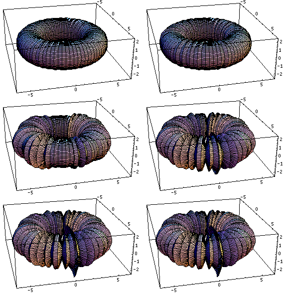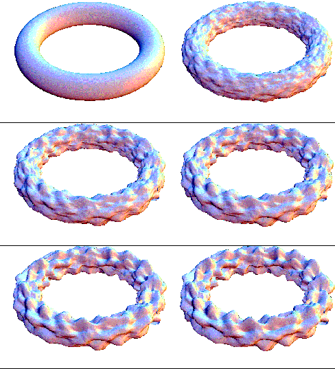
Turing was the first to suggest (in 1952) that the mechanisms of morphogenesis can be explained by reaction-diffusion equations. The idea is that each cell in a tissu (e.g. the skin) is characterized by two numbers, representing concentrations of substances (morphogens) a and b. The substances diffuse and react with each other following a partial differential equations of the form

where the vector-valued ![]() at each time t describes the changing spatial concentrations
of a and b. The function
at each time t describes the changing spatial concentrations
of a and b. The function  specifies the reaction and the laplacian term describes the diffusion.
Numerous variants have been studied and widely simulated. If one of the morphogen
is colored, these systems have been shown to produce regular patterns in
the tissu, reminiscent of zebra stripes and leopard spots. See here various
example of reaction-diffusion
patterns that can be produced. Turing's analysis stimulated considerable
theoretical research on mathematical models of pattern formation, but Turing-type
patterns were not observed in controlled laboratory experiments until 1990.
This kind of model have also been used not only to explain the marking on
animals, but reaction-riffusion processes have been used in areas such as:
Whether or not reaction-diffusion mechanisms are an actual phenomena in
such systems, simulation does tend to generate regular patterns that appear
as standing-wave solutions to the equations. This offers an explanation of
the breakdown of symmetry and homogeneity or the emergence of a pattern
in an originally homogenous medium.
We propose two examples coded in MGS in 1D and 2D.

This bubling torus is a visual representation of a diffusion-reaction process "à la Turing" on a ring of cells. A very simple MGS program is used to compute the density of two chemicals that diffuse and react on a ring of cells. The data are then written in a file together with a simple Mathematica program used to generate this plot. The diameter of the torus is proportional to the density of one of the chemicals.
|
specifying a reaction-diffusion in 1D
|
|
| gbf RING
= < d; 40 d = 0 >;; NbCell := 40;; |
Definition of a GBF
type. GBF means Group Based Fields. A GBF specifies a uniform
topology where the elements are indexed by a mathematical group. Here,
all elements in an instance of the GBF type RING has two
neighbors: one following the direction d and the other following
the inverse direction. If we go 40 steps following the direction d,
we reach again our starting point, hence the equation 40 d = 0.
This is juste the way in MGS to define a circural buffer (a ring of cells) and a displacement nammed d. |
| rsp := 1.0/16.0;; diff1 := 0.25;; diff2 := 0.0625;; fun da(a, b, la, ra) = rsp * (16.0 - a * b) + diff1*(la + ra - 2.0*a);; fun db(a, b, beta, lb, rb) = rsp*(a*b - b - beta) + diff2*(lb + rb - 2.0*b);; |
Definition of some constant
parameters. Definition of the function da and db that computes the change in a and b. Arguments a and b are the concentration in morphogen a and b at somme cell x, la is the concentration of morphogen a at the cell at left of x and ra the concentration at the cell at right of x. Identically for b, lb and rb. beta is a constant for each cell that introduces some fluctuations. |
| trans Turing = { x => let xl = hd('neighbor(x, <d|)) and xr = hd('neighbor(x, |d>)) in { a = x.a + da(x.a, x.b, xl.a, xr.a), b = max(0.0, x.b + db(x.a, x.b, x.beta, xl.b, xr.b)), beta = x.beta } };; |
The state of a cell is defined by a record x
containing the concentration in a, in b and the parameter beta.
The special function 'neighbor(x, dir) returns all the
neighbors of the cell x following the direction dir.
It returns a sequence. Here the sequence returned is a singleton (there is
only one neighbor following a given direction in a GBF) and we take this element
using hd (the head of the sequence). So, xl and xr denotes the element at the left and at the right of x. A new record is computed using the da and the db function to compute the new values of a and b. |
| trans init = { x => { a = 4.0, b = 4.0, beta = 12.0 + random(0.1) - 0.05 }; };; ring0 := init(iota(NbCell, ():seq) following |d>::seq:());; |
To compute an initial state, we apply the transformation init
to an initial ring. We do not care the elements in this ring, we rather replace
each element by a record containing some predefined value for the concentration
in a and b and a beta value which fluctuates around 12
+/- 0.05. The transformation init is applied to an initial ring obtained by coercing a sequence of 40 integer (computed by the function iota) into a ring. This coercion makes use of the function following. Following is an infix function that takes two arguments. The first argument is a sequences of elements and the second is a sequence of directions that specify the distribution of the elements into the ring. |
| Turing['iter=150](ring0) |
This expression computes 150 time steps of the process. |

|
the 2D diffusion-reaction
|
|
| gbf
torus = < a, b; 180 a,
60 b>;; NbCell_a := 180;; NbCell_b := 60;; |
Definition of a GBF
type. GBF means Group Based Fields. A GBF specifies a uniform
topology where the elements are indexed by a mathematical group. Here,
all elements in an instance of the GBF type torus has two
neighbors: one following the direction a, the other
following the direction b. (and also two others neighbors
reached following the inverse directions). If we go 180 steps following the
direction a, we reach again our starting point, hence
the equation 180 a = 0 which is abreviated as 180 a.
The same property holds for the direction b but after
60 steps. This is juste the way in MGS to define a circural 2D grid (a torus) whose dimensions are named a and b. |
| beta_init
:= 12;; beta_rand := 0.1;; u_steady := 4;; v_steady := 4;; diffu := 0.25 / 2.0;; diffv := 0.0625 / 2.0;; p1 := 0.2;; p2 := 0.0;; p3 := 0.0;; k := p1/16.0;; dt := 0.4;; |
Some consyant parameters are
declared (see the article of G. Turk for an explanation of these parameters). Each point if the torus is associated with a record with fields u, v and c. The first two fields record the concentration in morphogens.Think to this record as a vector. The field c is constant in timeand correspond to a perturbation term. |
| fun acc(r,
suite) = { u = r.u + suite.u, v = r.v + suite.v} ;; |
An auxilliary function is used
to compute the laplacian. This function simply make the pointwise sum of
the components u and v of two records. |
| trans Turing
= { x => let laplacian = neighborsfold(acc,{u= -4.0*x.u, v= -4.0*x.v},x) in let du = k * (16.0 - x.u*x.v) + diffu*laplacian.u and dv = k * (x.u * x.v - x.v - x.c) + diffv*laplacian.v in { u = x.u + dt*du, v = x.v + dt*dv, c = x.c } };; |
For each point x of the
torus, we compute the laplacian, which is simply a the sum of the neighbors
minus the current state at x (times an adequate factor).The
laplacian is then used to compute the increase in morphogens u and
v which are finally used to build the new state. |
| trans init = { x => { u = u_steady, v = v_steady, c = beta_init + random(2*beta_rand) - beta_rand } };; fun genere(n) = if n == 0 then seq:() else (iota(NbCell_a, ():seq))::genere(n-1) fi ;; torus0 := init(genere(NbCell_b) following |b>, |a>);; |
An auxilliary transformation init
is used to define an initial state. Starting from a torus, each element is
replaced by a record with fields u, v and c. The function genere is used to build a nested list. We don't care the element in the nested lists (they are generated by the iota function that gives a sequence of integers) The operator following is then used to convert this list into a torus and the transformation init is used to associate a record to each element of the toroidal grid. |
|
output of the simulation data |
|
| itere := 1400;; step := max(1, itere/40);; out := "tmp.2turing-" +NbCell_a +"-"+NbCell_b +"_"+itere+"_" +step+".m";; |
The simulation will evolve for
1400 time steps and a snapshot is taken every 40 iterations. The name of
the output file include the size of the torus, the number of iteration done
and the step. |
| fun Show(x)
= if 0 == ('iteration -1) % step then show[t='iteration](x) else Turing(x) fi ;; |
The function Show
is used to run the simulation. Parameter x is the current state.
The variable 'iteration is a contextual variable, managed by the
system and updated when the function Show is iterated (see below).
If the current iteration is a multiple of step, then the current
state is outputed to a file using the transformation show (Show
and show are two different names because capital letters are
meaningful in MGS). Else, an evolution step is made by applying the transformation Turing. |
| trans show[t=0] = { x => let pp = sequify(pos(x)) in let bx = take(pp, 0) and ax = take(pp, 1) in out << "dataTuring[" << t << "][" << ax << "][" << bx << "] = " << x.v << ";\n"; x };; |
The state of the torus is written
to a file using the transformation show. This transformation takes
an additional parameter t which represent the current time. Applied
on the torus, each element is selected by the only rule of this transformation. The position pos(x) of the element x is a word in the torus generator a and b. This word is transformed into a sequence of integers using the sequify function. The variables ax and bx represent the integer coordinates of this element in the circular grid along the axis a and b. And for each element, a line: dataTuring[t][ax][bx]
= v
(where v is the concentration of the morphogen of the element
x at time t) is written in the
output file.This file is then processed by a Mathematica program to visualize the torus. This visualization program in Mathematica makes use of the Tuba Mathematica package written by Prof. M A Berger. |
| Show['iter=itere](torus0);; |
The function is iterated starting from the initial
state torus0. |
| Back
to top |
MGS examples index |
MGS home page |

Pictures, graphics and animations are licensed under a Creative Commons License.
|
|