specifying the growth
|
state Position
= {x, y, z};;
state Cell = Position + {l};;
state Germ0 = Cell + {grow = 0};;
state Germ1 = Cell + {grow = 1};;
|
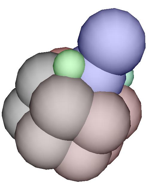
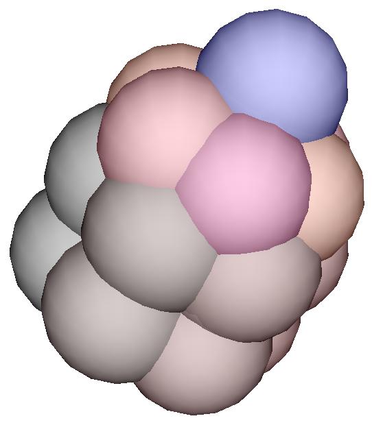
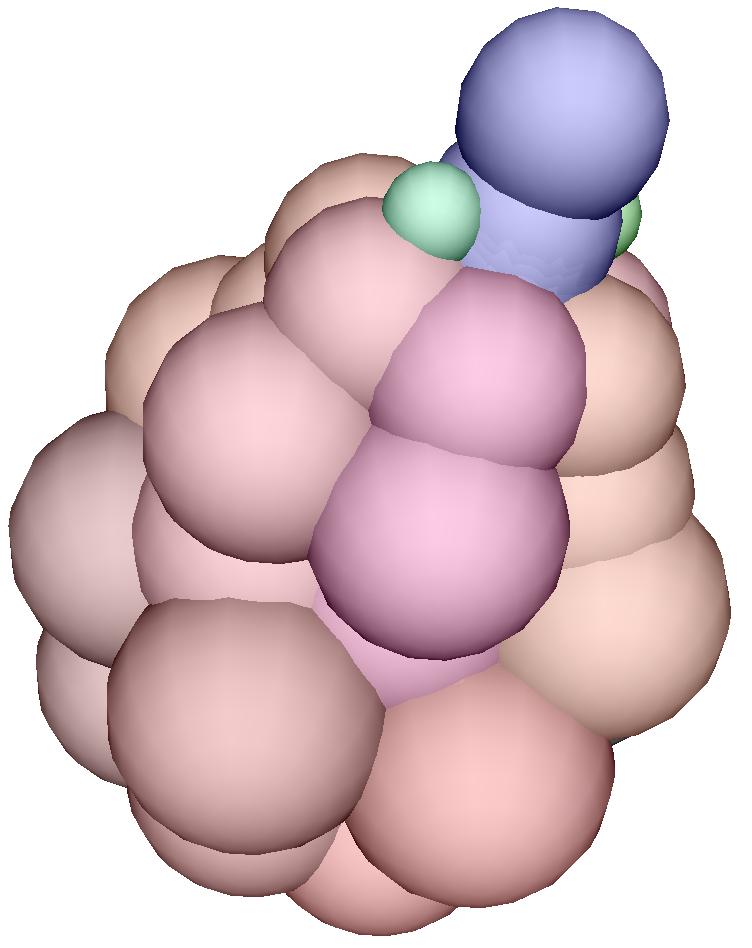
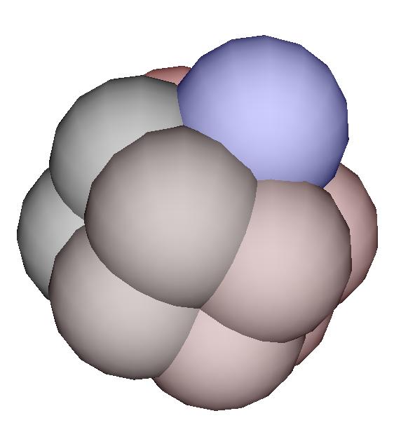
A cell is decribed by a record
that contains the fields necessary to be a Position (i.e. three
fields named x, y and z) and a stiffness coefficient
l. A cell is also "alive" if it has in addition a field called
grow. If this field has the value 0, then the cell is ready
to divide (blue cell). If the field has the value 1, then the cell
is a green cell and will divide into 3 vegetative cells. If this fields has
a negative value n, then the cell will be ready to divide after
waiting n time steps.
|
delaunay(3) D3
=
\e.if Position(e)
then (e.x, e.y, e.z)
else ?("bad element type for D3 delaunay type")
fi
;;
|
This function extract a position
from a cell record and is used in the definition of the Delaunay collection
type that represents the spatial organization of the meristeme.
|
epsilon := 0.05;;
K := 1.0;;
|
Some constant parameter of the mechanical part of
the model are defined.
|
fun interaction(ref,
src) =
if(Cell(ref) && Cell(src)) then
(
let X = ref.x - src.x
and Y = ref.y - src.y
and Z = ref.z - src.z
and L = ref.l + src.l
in let dist = sqrt(X*X+Y*Y+Z*Z)
in let force = 0.0-K*(dist-L)/dist
in {x=X*force, y =
Y*force, z = Z*force}
)
else
?("Error : bad argument type for interaction/2");
?(ref); ?(src); ?("Et voil� ...")
fi
;;
fun add(u, v, e) = u + { x = u.x + e*v.x,
y = u.y + e*v.y,
z = u.z + e*v.z }
;;
fun sum(x, u, acc) = add(acc, interaction(x,u), 0.05)
;;
trans Meca =
{
x => add(x,neighborsfold(sum(x), {x=0,y=0,z=0, l=x.l}, x), epsilon)
};;
|
These functions and the transformation
Meca compute the mechanical interaction between two neighboring
cells. For a more detailed explanation, see here.
|
p1 := 0;;
p2 := PI/3;;
p3 := 2*PI/3;;
p4 := PI;;
p5 := 4*PI/3;;
p6 := 5*PI/3;;
alpha := 5.0;;
theta := PI/6;;
theta2 := PI/3;;
|
Now we will specify the growing process. We defines
some angles that are used to position the cell when they appear.
Note that this model is a phenomenological one: it describes a (rough) sketch
of the observed growth and for example, it does not explain the emergence
of a phylotactic spiral from low-level interactions.
|
trans Grow =
{
r / r.grow < 0
=> r + {grow = r.grow+1 };
r/ r.grow == 0
=>
r+{z = r.z + alpha, grow = -5},
r+{x = alpha*cos(p1+theta), y = alpha*sin(p1+theta),
grow=1, l = r.l/2, color = "Color<0, 1.0,
0.0>"},
r+{x = alpha*cos(p4+theta), y = alpha*sin(p4+theta),
grow=1, l = r.l/2, color = "Color<0,
1.0, 0.5>"};
r/r.grow == 1
=>
r+{x=r.x+0.2, y=r.y+0.2,
l = r.l*2, grow=2, color = "Color<1.0,
0.2, 0.3>"},
r+{x=r.x*cos(theta2)-r.y*sin(theta2),
y = r.x*sin(theta2) + r.y*cos(theta2),
l = 2*r.l, grow=2, color
= "Color<1.0, 0, 0.5>"},
r+{x=r.x*cos(0.0-theta2)-r.y*sin(0.0-theta2),
y = r.x*sin(0.0-theta2) + r.y*cos(0.0-theta2),
l = 2*r.l, grow=2, color
= "Color<1.0, 0.3, 0.1>"};
r/r.grow == 2
=> r + {l=r.l+0.15};
};;
|
The growth is specified by 4 rules:
- The first rule specifies that an alive cell in a waiting state
(grow < 0) simply wait some time. Its evolution consists simply
in increasing the field grow: then at next time steps there is little
time to wait. The operator + that appears between records compute
the asymetric merge of its argument.
- The second rule specifies that a ready blue cell (grow =
0) divide into 3 new cells: a blue one and two green (grow=1).
- A green cell divides into 3 vegetative cells
- A vegetative cell (grow = 2) simply increase in size.
The field color is used to specify the color of the cell in the
graphical representation.
|
fun H(d) =
let dd = Meca[20](d) in
let s = sequify(dd) in
let ns = Grow(s) in
delaunayfy(D3:(), ns)
;;
|
An evolution of the system is simply 20 steps of the
mechanical evolution Meca followed by one steps of growth.
For some obscure reasons, the meristem (which is a Delaunay collection) is
turned into a sequence (operator sequify) befor applying the growth
and then is turned back into a Delaunay collection (operator Delaunayfy).
This step can be avoided.
|
building the initial state
|
pre_init
:=
{x = alpha*cos(p1), y = alpha*sin(p1), z = 0.01, color = "Color<0.0,
0, 0>", l = alpha, grow=2},
{x = alpha*cos(p2), y = alpha*sin(p2), z = 0.02, color = "Color<0.2,
0, 0>", l = alpha, grow=2},
{x = alpha*cos(p3), y = alpha*sin(p3), z = 0.00, color = "Color<0.4,
0, 0>", l = alpha, grow=2},
{x = alpha*cos(p4), y = alpha*sin(p4), z = 0.01, color = "Color<0.6,
0, 0>", l = alpha, grow=2},
{x = alpha*cos(p5), y = alpha*sin(p5), z = 0.03, color = "Color<0.8,
0, 0>", l = alpha, grow=2},
{x = alpha*cos(p6), y = alpha*sin(p6), z = 0.02, color = "Color<1.0,
0, 0>", l = alpha, grow=2},
{x = alpha*cos(p1), y = alpha*sin(p1), z = 5.01, color = "Color<0.0,
0, 0>", l = alpha, grow=2},
{x = alpha*cos(p2), y = alpha*sin(p2), z = 5.02, color = "Color<0.2,
0, 0>", l = alpha, grow=2},
{x = alpha*cos(p3), y = alpha*sin(p3), z = 5.00, color = "Color<0.4,
0, 0>", l = alpha, grow=2},
{x = alpha*cos(p4), y = alpha*sin(p4), z = 5.01, color = "Color<0.6,
0, 0>", l = alpha, grow=2},
{x = alpha*cos(p5), y = alpha*sin(p5), z = 5.03, color = "Color<0.8,
0, 0>", l = alpha, grow=2},
{x = alpha*cos(p6), y = alpha*sin(p6), z = 5.02, color = "Color<1.0,
0, 0>", l = alpha, grow=2},
{x = 0, y = 0, z = 10.0, color = "Color<0, 0, 1.0>", l = alpha,
grow = 0}
;;
|
We build an initial description
of the meristem simply by listing the state of its cells...
|
init := delaunayfy(D3:(), pre_init)
;;
|
... and then computing its spatial organization
by a Delaunay triangulation.
|
|
|
the graphical output
|
outfile := "tmp.moving1.imo";;
|
The previous pictures are generated
by specifying a 3D scene in TEOM. TEOM is a 3D description language
described here.
|
fun show_line(a, b, acc) = (
outfile << "Polyline { PointList
[ <" + a.x + ", " << a.y << ", " << a.z << ">,
<"
<< b.x << ", " <<
b.y << ", " << b.z << "> ]}\n";
acc )
;;
|
A detailed comment of generation of the scene description
can be found here.
|
trans show_edge = {
x => (neighborsfold(show_line(x), 0, x); x)
}
;;
|
|
fun show_cell(a) =
"Translated { Translation <"
+ a.x + ", " + a.y + ", " + a.z
+ "> Geometry Sphere { Radius "
+ a.l/1.0 + " Slices 16 Stacks 16 "
+ a.color + "} }"
;;
|
|
cpt := -1;;
fun show(f, c) = (
cpt := 1+cpt;
if 0 == cpt % 1 then (
print_coll(f, c, show_cell,
"Group { GeometryList [\n\t",
",\n\t",
"\n] }\n\nCommand Pause\n\n"))
else
0
fi)
;;
|
|
fun evol(xxx) = (show(outfile, xxx);
H(xxx))
;;
evol[20](init);;
system("imoview "+outfile);;
|
|
 Click on the picture to enlarge the view.