
The cyanobacterium Anabaena grows in filaments of 100 cells or
more. When starved for nitrogen, specialized cells called heterocysts
differentiate from the photosynthetic vegetative cells at regular intervals
along each filament. Heterocysts are anaerobic factories for nitrogen fixation;
in them, the nitrogenase enzyme complex is synthesized and the components
of the oxygen-evolving photosystem II are turned off. Plant signals exert
both positive and negative regulatory control on heterocyst differentiation.
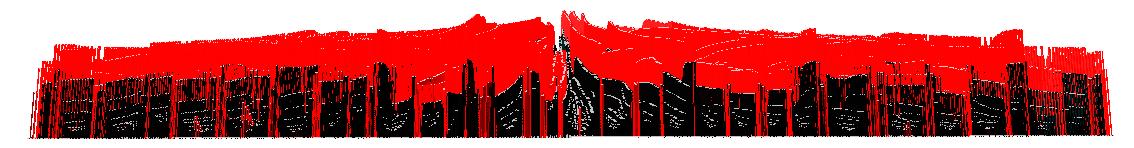
In the upper graphic, the time goes from left-upper to righ-lower corner.
Each slice (lower graphic) corresponds to the state of a growing filament
and represent a sequence of cells. The height of a cell represent the
activator concentration. Cells are pictured in red when the activator
is greater than a given level triggering differentiation (they are in pale
gray above). Black cells are vegetative ones. This type of visualization,
called ``space-time extrusion'' has been developped in (Hammel 1996).
|
Specifying the anabaena growth
|
|
| record
CellState = { a, h, x, p, type };; record C = { a, h, x, p, type = "C"};; record D = CellState + { type = "D" };; |
The state of a cell is given
by a record (a struct in C) with five fields: a is the activator
concentration (in the cell) and h is the inhibitor concentration.
Field x represents the size of the cell and p is the polarity.
Each cell is either vegetative or heterocyst has indicated by the field type. The type C and D are specialization of CellState and specify that the cell is vegetative (the field type has the value "C") or heterocyst (e.g.: differentiated and the field type has the value "D"). The system will be composed of a sequence of such states. |
| LM
:= 0;; RM := 1;; longer := 0.61803;; shorter := 0.38196;; rho := 3.0;; a0 := 0.01;; mu := 0.1;; Da := 0.0000;; h0 := 0.001;; nu := 0.45;; Dh := 0.004;; kappa := 0.001;; dt := 0.1;; w := 0.01;; lm := 1.0;; gr := 1.002;; thr := 1.0;; |
Definitions of some constants
and parameters. LeftMark and RightMark are symbols used to indicate the polarity of a cell. longer is the elongation factor when a cell grows and shorter is the corresponding shrinking factor. lm is the threshold on the size for the cell division (a cell must be big enough to divide). |
| trans
T = { |
|
| e / (C(e)
& (e.x >= lm) & (e.p == RM)) => {type="C", a=e.a, h=e.h, x= e.x*longer, p=LM}, {type="C", a=e.a, h=e.h, x= e.x*shorter, p=RM}; |
This rule specifies when a cell
with a left polarity divides. Only vegetative cell can divided (hence the predicate C in the rule guard) and it must be big enough. The volume of the two daughter cells remains the same, so there is no variation in the concentration. |
| e / (C(e)
& (e.x >= lm) & (e.p == LM)) => {type="C", a=e.a, h=e.h, x=e.x*shorter, p=LM}, {type="C", a=e.a, h=e.h, x=e.x*longer, p=RM}; |
This rule specifies when a cell
with a right polarity divides. |
| e / (C(e)
& C(left(e)) & C(right(e))) => begin let al = left(e).a and ar = right(e).a and hl = left(e).h and hr = right(e).h in let h = e.h and a = e.a and x = e.x and p = e.p in { type = "D", a = a + (rho/h*(a*a/(1+kappa*a*a) + a0) - mu*a + Da*(al+ar-2*a)/(x*w))*dt, h = h + (rho*(a*a/(1+kappa*a*a) + h0) - nu*h + Dh*(hl+hr-2*h)/(x*w))*dt, x = x, p = p} end; |
When a cell does not divide, the
concentration in activator and inhibitor evolves following some kinetics rules.
Cf. (Hammel1996). The operator left and right are used to access the left and right neighbors of an element in a sequence. |
| p4 = e / (D(e)
& (e.a >= thr) & (e.x < shorter*gr)) => {type ="C", a=e.a, h=e.h, x=e.x, p=e.p}; |
The two following rules state that
a differentiated cell returns to a vegetative state if it is too small or
if the concentration of the activator is too low. |
| e / (D(e)
& (e.a < thr) | (e.x >= shorter*gr)) => {type ="C", a=e.a/gr, h=e.h/gr, x=e.x*gr, p=e.p}; |
In addition, if the cell is big
enough, it continues to grow. |
| e / C(e) => {type="D", a=e.a, h=e.h, x=e.x, p=e.p}; |
A vegetative cell that does not
meet the previous constraints becomes an heterocyst. |
| };; |
|
| omega := {type="C", a=0.1, h=10.0, x=0.5, p=RM}, seq:();; |
The initial condition : a filement composed of one
cell. |
Visualization |
|
| fun pre_exec(fichier)
= fichier << "Scaled{ Scale <0.1, 0.1, 0.1>\n Geometry Grid1{ Axis<1,0,0> LineUp2 Middle GridList[" ;; |
The following functions are
used to writte in a file a 3D graphical description of the picture above. The 3D description language is described here. The function pre_exec is used to produce the head of the description file. |
| fun post_exec(fichier)
= fichier << "Box { Size <0, 0, 0>} \n] }}\n" ;; |
The function post_exec
is used to produce the end of the description file. |
| fun every(fichier,
l, nb) = if ((nb % 5) == 0) then (fichier << "Grid1{Axis<0,0,1> Space1 0.1 GridList["; map(show(fichier), l); fichier << "Box { Size <0, 0, 0>} ] },\n") else 0 fi ;;x |
The function every
is used to produce the description of the current state. This function is
called at each time steps but a description is outputed to the file only every
5 calls. The current state is a sequence of box, one box per cell. The height
of this box is proportional to the concentration of the activator. The description
of the box is produced by a call to the function show.
|
| fun show(fichier, e) =
fichier << "Box { Size <0.15, " << sqrt(e.h/2.0) << ", " << e.x/2.0 << "> Color < " << e.a / 8.0 << ", " << e.a / 8.0 << ", " << e.a / 8.0 << "> },\n";; |
|
| fun simul(x)= begin pre_exec("ana.output"); evolve(nb, x) ; post_exec("ana.output") end;; fun evolve(nb, x) = if (nb == 0) then (?("\nAnaeba final size: " + size(x) + "\n"); x) else (every("ana.output", x, nb); evolve(nb-1, T(x))) fi ;; simul(5000, omega);; |
A simulation consists in outputing
the head of the data file, outputing the description of the current state
and the outputing the end of the data file. The image below corresponds to a simulation over 5000 time steps. |
| Back
to top |
MGS examples index |
MGS home page |

Pictures, graphics and animations are licensed under a Creative Commons License.
|
|
|